吴恩达机器学习实验（三）

多分类任务

上一讲中涉及到的Logistic回归是二分类问题，即每一次分类只能完成0-1分类的任务，但是我们也提到过，如果有k个种类，我们可以采用Logistic方法分割四次来解决问题，例如这个分类任务:

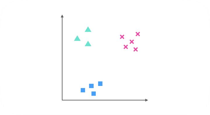
显然，有三个类别，我们可以采用Logistic回归做如下三次分类：

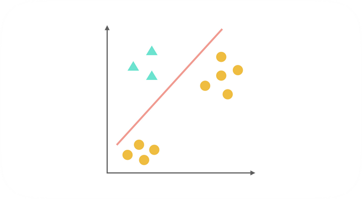
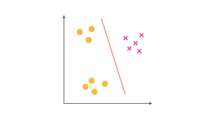
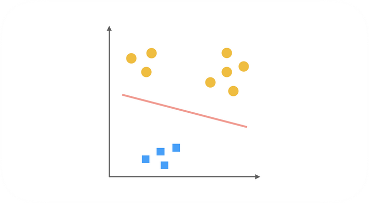
综上，得到了三种二元分类器。在预测阶段，每个分类器根据测试样本得到当前正类（即单独的上图中非黄色的一类）的概率。选择计算结果最高的分类器，其正类就可以作为预测结果。

神经网络

之前涉及的线性回归和Logistic回归都存在一个问题，即当特征数量很多时，计算负荷会变得特别大。这也是传统机器学习算法一般都具有的问题，例如在图片当中，每个像素点都是一个特征，这对于传统的机器学习是很难解决的。为了应对这种问题，科学家仿照人脑中神经元处理信息的模式，创造了神经网络。

神经网络建立在很多神经元上，每个神经元都是一个处理单元，具有一个激活函数，用来处理接收到的特征，每个神经元有多个输入（类比树突），代表着该神经元接收到了多个特征，每个神经元有一个输出（类比轴突），代表着经过激活函数处理的多种特征的合并，可以理解为对特征进行了提取和改造。其中的轴突和树突（即连接神经元的边）代表着不同的权重。

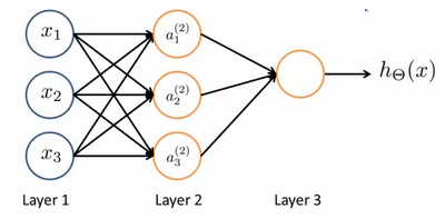
如上图是一个简单的三层神经网络，分为输入层、隐藏层和输出层，输入层就是最原始的特征，每个特征经过加权和喂到了中间层，然后中间层神经元的激活函数对其进行处理，再一次加权送到输出层，这就是前向传播的过程。其中，像之前设计偏置项一样，我们也会为每一层新添一个神经元，做为偏置项：

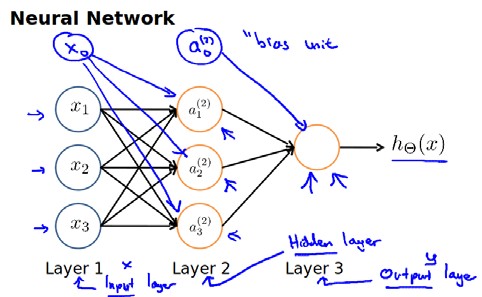
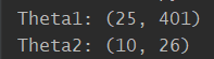
注意，每条边都代表着一个权重，那么我们的参数矩阵$\Theta$要求行数是下一层的神经元个数，列数是本层神经元个数加一。

上图所示的模型，激活单元和输出分别为：

$a_{1}^{(2)}=g(\Theta _{10}^{(1)}{x_0}+\Theta _{11}^{(1)}{x_1}+\Theta _{12}^{(1)}{x_2}+\Theta _{13}^{(1)}{x_3})$
$a_2^{(2)}=g(\Theta _{20}^{(1)}{x_0}+\Theta _{21}^{(1)}{x_1}+\Theta _{22}^{(1)}{x_2}+\Theta _{23}^{(1)}{x_3})$
$a_3^{(2)}=g(\Theta _{30}^{(1)}{x_0}+\Theta _{31}^{(1)}{x_1}+\Theta _{32}^{(1)}{x_2}+\Theta _{33}^{(1)}{x_3})$
$h_{\Theta}(x)=g(\Theta _{10}^{(2)}a_0^{(2)}+\Theta _{11}^{(2)}a_1^{(2)}+\Theta _{12}^{(2)}a_2^{(2)}+\Theta _{13}^{(2)}a_3^{(2)})$

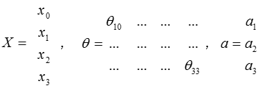
这只是考虑一个3维的数据样本，若$X$为数据集，$\Theta$为网络参数，$a$为输出，可以得到：

$\Theta ·X = a$

实验描述

实验一

For this exercise, you will use logistic regression and neural networks to recognize handwritten digits (from 0 to 9). Automated handwritten digit recognition is widely used today - from recognizing zip codes (postal codes) on mail envelopes to recognizing amounts written on bank checks.

本次实验直接采用scipy中optimize模块中的minimize函数来对损失函数进行优化，与上一个实验不同的地方在于，同时求所有变量的梯度：

# 整体同时求梯度
def gradient(theta, X, y, learning_rate):
    error = sigmoid(np.dot(X, theta.T)) - y
    grad = (np.dot(X.T, error) / y.shape[0]).T + ((learning_rate / y.shape[0]) * theta)
    grad = grad.reshape((-1, 1))
    grad[0, 0] = np.sum(error * X[:, 0]) / y.shape[0]
    return grad.ravel()

构造k个分类器的函数如下：

def one_vs_all(X, y, k, learning_rate):
    """
    分类器函数
    :param X: 输入数据，5000 x 400
    :param y: 数据对应的标签，5000 x 1
    :param k: 需要分类的数量，本次实验k=10（1，2，...,10一共10个数字）
    :param learning_rate: 学习率，为惩罚项的系数
    :return: all_theta矩阵，每一行是每个分类的所有参数
    """
    m = y.shape[0]  # 样本数量
    params = X.shape[1]  # 参数数量
    all_theta = np.zeros((k, params+1))    # k x 401（多出的1为截距）
    X = np.concatenate((np.ones(m).reshape((m, 1)), X), axis=1)  # 扩充了np.ones((5000, 1))

    # 分别构造k个分类器
    for i in range(1, k + 1):
        theta = np.zeros(params + 1).reshape((1, -1))
        y_i = np.array([1 if label == i else 0 for label in y])
        y_i.reshape((m, 1))
        fmin = minimize(fun=cost, x0=theta, args=(X, y_i, learning_rate), method='TNC', jac=gradient)
        all_theta[i-1, :] = fmin.x
    return all_theta

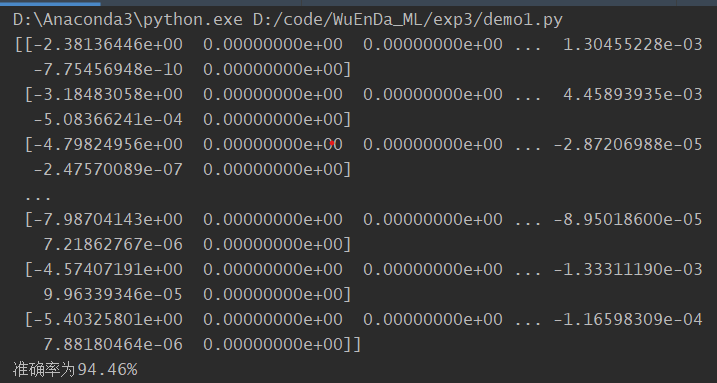
模型准确率为94.46%。

实验二

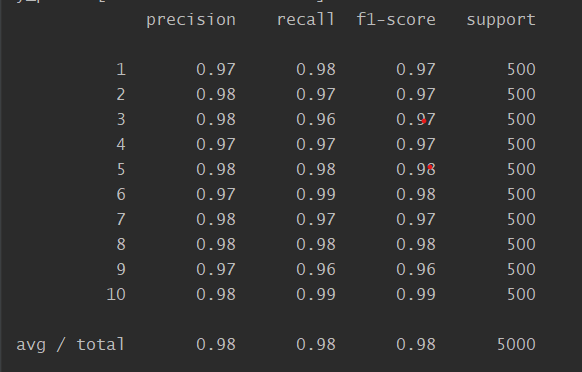
In this part of the exercise, you will implement a neural network to recognize handwritten digits using the same training set as before.Your goal is to implement the feedforward propagation algorithm to use our weights for prediction.

本次实验比较简单，只需要简单地完成前向传播的过程即可。网络参数已经训练好，关键是把握好矩阵乘法的维度和添加偏置项：

实验代码

实验一

import numpy as np
from scipy.io import loadmat
from scipy.optimize import minimize

data = loadmat('ex3data1.mat')
X = data['X']
y = data['y']


def sigmoid(z):
    return 1 / (1+np.exp(-z))


def cost(theta, X, y, learning_rate):   # learning_rate为控制惩罚项的参数
    y = y.reshape((-1, 1))
    theta = theta.reshape((1, -1))
    first = -y*np.log(sigmoid(np.dot(X, theta.T)))
    second = -(1-y)*np.log(1-sigmoid(np.dot(X, theta.T)))
    punish = np.sum(np.power(theta[:, 1:theta.shape[1]], 2))*learning_rate/(2*y.shape[0])
    return np.sum(first+second)/y.shape[0] + punish


# 整体同时求梯度
def gradient(theta, X, y, learning_rate):
    error = sigmoid(np.dot(X, theta.T)) - y
    grad = (np.dot(X.T, error) / y.shape[0]).T + ((learning_rate / y.shape[0]) * theta)
    grad = grad.reshape((-1, 1))
    grad[0, 0] = np.sum(error * X[:, 0]) / y.shape[0]
    return grad.ravel()


def one_vs_all(X, y, k, learning_rate):
    """
    分类器函数
    :param X: 输入数据，5000 x 400
    :param y: 数据对应的标签，5000 x 1
    :param k: 需要分类的数量，本次实验k=10（1，2，...,10一共10个数字）
    :param learning_rate: 学习率，为惩罚项的系数
    :return: all_theta矩阵，每一行是每个分类的所有参数
    """
    m = y.shape[0]  # 样本数量
    params = X.shape[1]  # 参数数量
    all_theta = np.zeros((k, params+1))    # k x 401（多出的1为截距）
    X = np.concatenate((np.ones(m).reshape((m, 1)), X), axis=1)  # 扩充了np.ones((5000, 1))

    # 分别构造k个分类器
    for i in range(1, k + 1):
        theta = np.zeros(params + 1).reshape((1, -1))
        y_i = np.array([1 if label == i else 0 for label in y])
        y_i.reshape((m, 1))
        fmin = minimize(fun=cost, x0=theta, args=(X, y_i, learning_rate), method='TNC', jac=gradient)
        all_theta[i-1, :] = fmin.x
    return all_theta


all_theta = one_vs_all(X, y, 10, 1)
print(all_theta)


# 输出预测结果
def predict(X, all_theta):
    m = y.shape[0]
    X = np.concatenate((np.ones(m).reshape((m, 1)), X), axis=1)
    tmp = sigmoid(np.dot(X, all_theta.T))
    pred = (np.argmax(tmp, axis=1) + np.ones(m)).reshape((-1, 1))
    return pred


y_pred = predict(X, all_theta)  # 预测结果
count = 0   # 计算预测错误的样本个数
for (a, b) in zip(y_pred, y):
    if a != b:
        count += 1
print('准确率为%.2f%%' % ((1-count/y.shape[0])*100))

实验二

import numpy as np
import scipy.io as sio
from sklearn.metrics import classification_report  #这个包是评价报告

def sigmoid(z):
    return 1 / (1+np.exp(-z))


data = sio.loadmat('ex3data1.mat')
X = data['X']
y = data['y']
weights = sio.loadmat('ex3weights.mat')
Theta1 = weights.get('Theta1')
Theta2 = weights.get('Theta2')
print('Theta1:', Theta1.shape)
print('Theta2:', Theta2.shape)

m = y.shape[0]

X_1 = np.concatenate((np.ones(m).reshape((m, 1)), X), axis=1)
X_2 = np.dot(X_1, Theta1.T)
X_2 = sigmoid(np.concatenate((np.ones(m).reshape((m, 1)), X_2), axis=1))
y_pred = sigmoid(np.dot(X_2, Theta2.T))
y_pred = np.argmax(y_pred, axis=1) + 1
print('y_pred:', y_pred)
print(classification_report(y, y_pred))