Logistic回归
Logistic回归(Logistic Regression)虽然名字叫“回归”,但实际是一种最经典的二元分类算法。在分类问题中,我们的输出是一个类别,例如收到的邮件是否是垃圾邮件,肿瘤是否是阳性的等等。
Logistic回归最大的特点在于引入了sigmoid函数(又称为logistic函数):
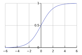
sigmoid函数能将输入变量展平到(0,1)的区间,我们很容易联想到概率,即划分为两个子类(1和0)的概率可以用sigmoid函数的输出值来表示。因此,我们可以拟合一条分割曲线,将输入数据喂入分割曲线,得到的数值作为sigmoid函数的自变量,即大于0代表分类为1,否则分类为0。我们采用sigmoid函数的另一大优势是sigmoid函数的导数形式很简洁。
代价函数
我们如果依旧采用平方误差函数作为代价函数,将sigmoid函数代入后发现,我们需要优化的代价函数变成了非凸的,这样不方便我们求解。因此我们选择采用信心论中常用的信息熵的方法来通过概率值(sigmoid函数输出值)衡量信息量的大小。
我们定义cost function为:
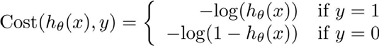
这样cost的曲线为:
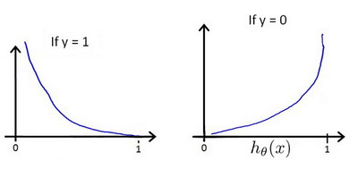
很容易看出,若标签为1,当数据的sigmoid输出越接近1,cost值越小,反之,若标签为0,当数据的sigmoid输出越接近0,cost值同样越小。所以这个cost function很好的反映了数据和标签的关系。
cost function可以化简如下:
代入代价函数为:
得到了代价函数后,我们采用梯度下降的方法来更新参数,达到最小化代价函数的目的:
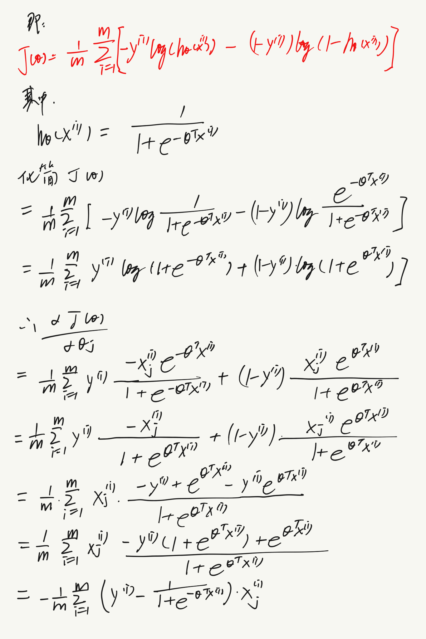
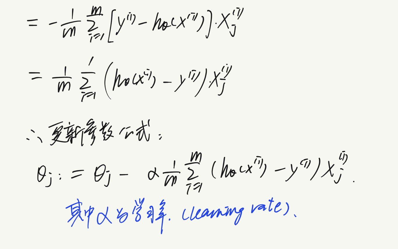
求导后得到:
注意!!!其中的$\theta$更新依然是同时更新所有的值,所以写代码时需要在这里新开辟一个列表或矩阵存储暂时的$\theta_j$
实验描述
实验一
Suppose that you are the administrator of a university department and you want to determine each applicant’s chance of admission based on their results on two exams. You have historical data from previous applicants that you can use as a training set for logistic regression. For each training example, you have the applicant’s scores on two exams and the admissions decision. Your task is to build a classification model that estimates an applicant’s probability of admission based the scores from those two exams.
- 首先我们读取数据
1 | with open('ex2data1.txt', 'r') as f: |
打印出数据散点图:
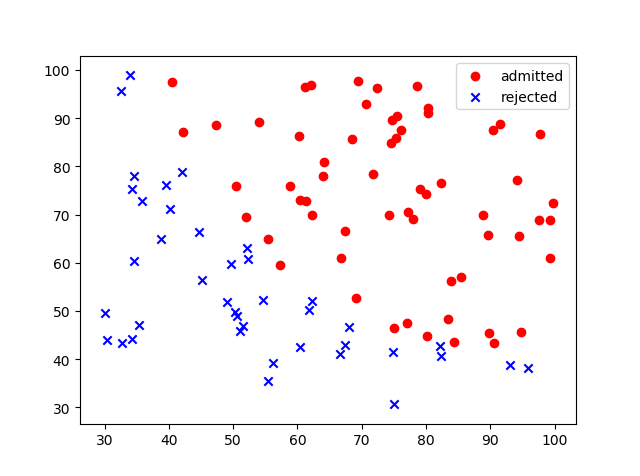
可以看出,我们大致可以用一条直线来分割数据。
- 构造矩阵,初始化参数
1 | # 构造数据和标签矩阵 |
- 编写sigmoid函数
1 | def sigmoid(X, theta): |
- 编写cost function
1 | def compute_cost(X, y, theta): |
其中对数函数默认为自然对数。
- 编写梯度下降函数
1 | def gradient_descent(X, y, theta, alpha): |
这次我规定当cost的变化量小于0.0001时停止迭代。
- 打印训练过程,并编写测试器分类准确度函数
1 | theta, cost, ite = gradient_descent(X, y, theta, alpha) |
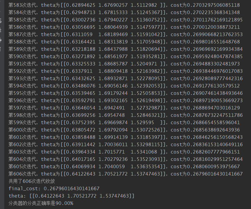
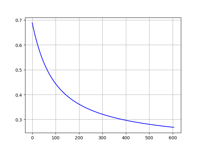
可以看到我们分类器的正确率为90%。
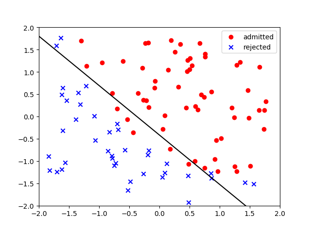
- cost训练曲线和分类结果
实验二
Suppose you are the product manager of the factory and you have the test results for some microchips on two different tests. From these two tests, you would like to determine whether the microchips should be accepted or rejected.
- 首先做出数据的散点图:
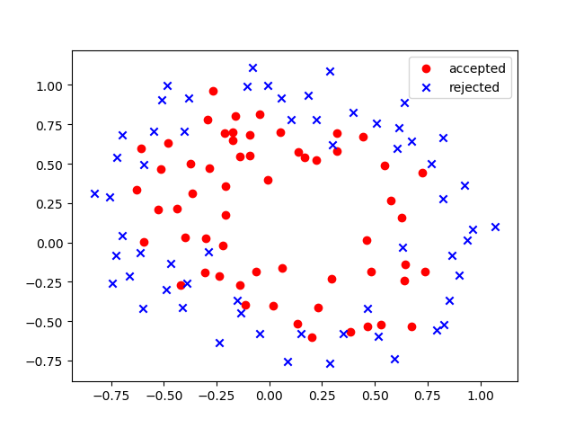
我们可以看出两类数据明显是无法用线性分类器分开的,但是近似可以用一个椭圆来区分,因此我们将$(x_1,x_2,x_1^2,x_2^2)$作为五个特征,这样可以转换非线性分类器为线性分类器。
- 为了防止过拟合,我这次采用添加了惩罚项的cost function:
1 | def compute_cost(X, y, theta, lam): |
可以看出我添加了一项惩罚项,目的是防止$\theta$值过大,造成过拟合,现在的cost function变成了:
- 编写梯度下降函数
由于添加了正则项,在更新参数的过程中每次还要加上$\frac{\lambda}{m}\theta_j$(除了$\theta_0$,因为我们未对其正则化)。
1 | def gradient_descent(X, y, theta, alpha): |
- 查看结果,做出cost下降曲线
1 | theta, cost, ite = gradient_descent(X, y, theta, alpha) |
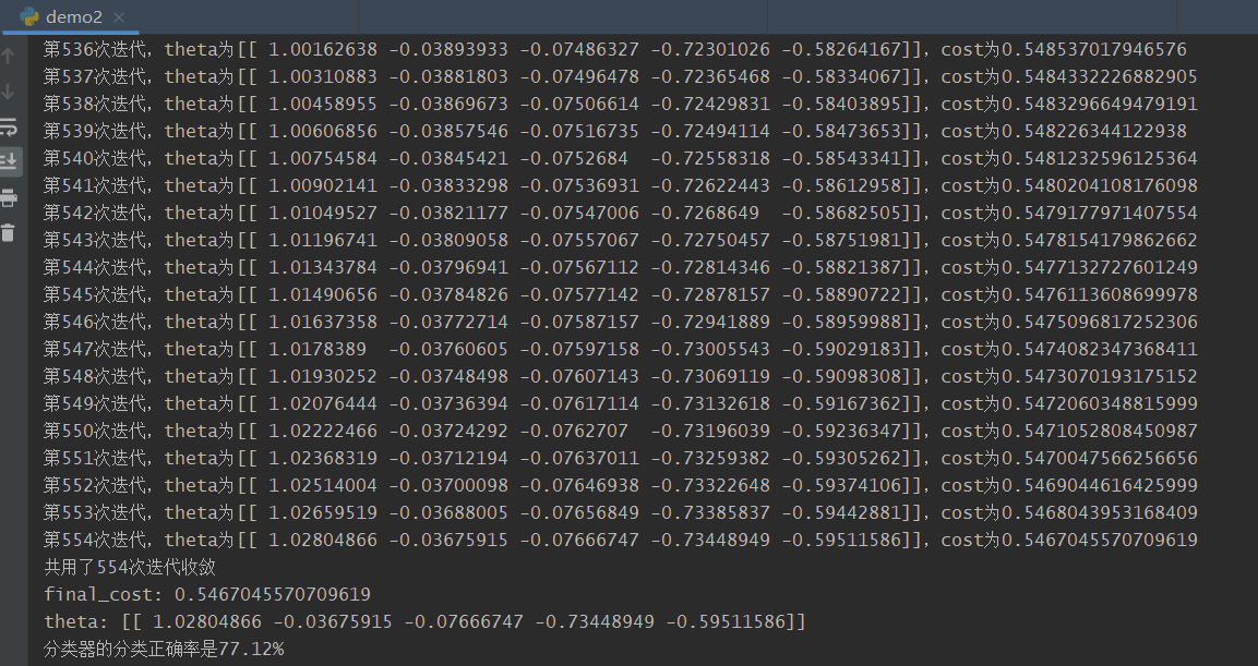
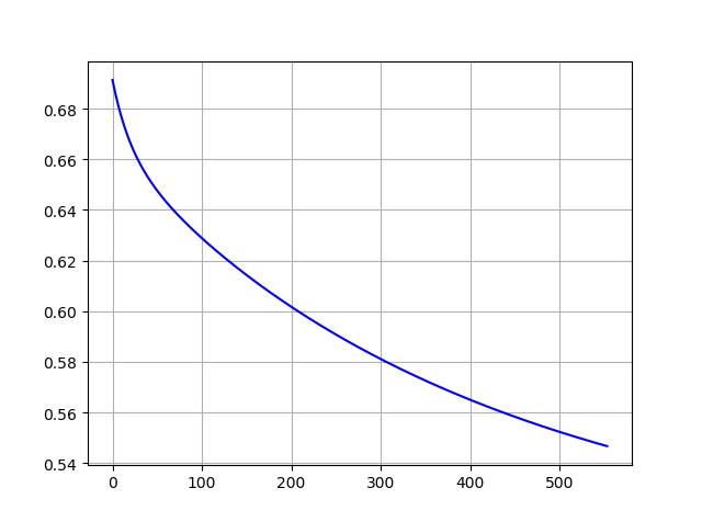
分类器正确率为77.12%。
cost下降曲线:
实验问题
最大的问题集中在数学推导信息熵的导数以及利用经过特征缩放的数据拟合出的曲线的参数和实际参数的关系。后者还未解决。
完整代码
1 | import numpy as np |