线性回归
线性回归(Linear Regression)是回归问题,回归是一种最常见的监督学习的方式,目的是预测,即给定数据集和对应的标签,训练一个回归函数,当喂进来新的数据时,利用我们训练好的函数来计算输出结果。而线性回归就是用直线去拟合数据。
需要注意的是,并非所有的数据都可以用直线来拟合对于某些数据,我们做出大致的散点图可以看出并非是一条直线,但是我们可以通过对于特征的变化将其变为直线拟合,例如输出值是关于特征a的二次函数(近似),我们可以采用二次函数来拟合,也可以构建输出值与$a^2$的关系,这样就可以用直线来拟合。
另一个需要注意的点是,我们的数据的特征单位不同,因此有时无法在一个维度来考虑,例如想通过房子的面积、卧室数量等等特征来预测房子的价格,但是房子的面积通常在100-200附近,而房间的卧室的数量则在1-4附近,因为单位不同而试图去拟合往往需要更长的时间才能使拟合的曲线收敛,因此我们通常会采用
的方式将特征的值移动到[-1, 1]附近。
梯度下降
拟合的本质是最小化代价函数,代价函数是就是通过预测器预测的结果和标签的差异,本次实验我们采用平方误差函数作为代价函数,即:
我们需要不断调整$\theta_0$和$\theta_1$的值来最小化我们的代价函数,梯度下降是一种求函数最小值的常用算法。我们考虑从曲线上一点开始寻找曲线的最小值,梯度指的是沿着某个变量的方向,即某个点的曲线切线斜率,梯度下降就是我们每次沿着这个方向走一个步长。若离最小点远,此时斜率自然大,那么我们用步长$\alpha$乘以梯度就大,我们向最小点移动的距离也就长;若离最小点近,此时斜率自然小,那么我们用步长$\alpha$乘以梯度就小,我们向最小点移动的距离就短,因此我们无需调整步长(或称为学习率)的大小。
- 批量梯度下降(batch gradient descent)
将全部数据同时用来训练预测器,每次计算全部参数的变化(求偏导),然后再同时更新。(注意顺序)
实验描述
数据集“ex1data1.txt”给出的第一列是城市人口,第二列是利润。我们需要用这些数据来预测新的城市的利润。
- 首先我们读取数据,并转化成矩阵
1 | with open('ex1data1.txt', 'r') as f: |
- 然后我们编写计算代价的函数
1 | # 计算代价函数 |
- 接着编写梯度下降的函数
1 | # 梯度下降 |
我本次设置迭代次数为1000次,也可以设置一个阈值,当新的代价和上一次迭代的代价的差小于阈值时停止迭代。
- 得到结果,做出图像
1 | # alpha设为0.01 |
这是最后几次迭代的代价变化:
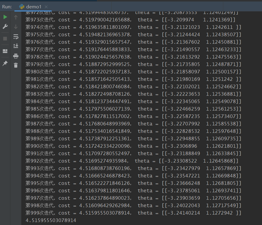
最终的cost为4.51596。
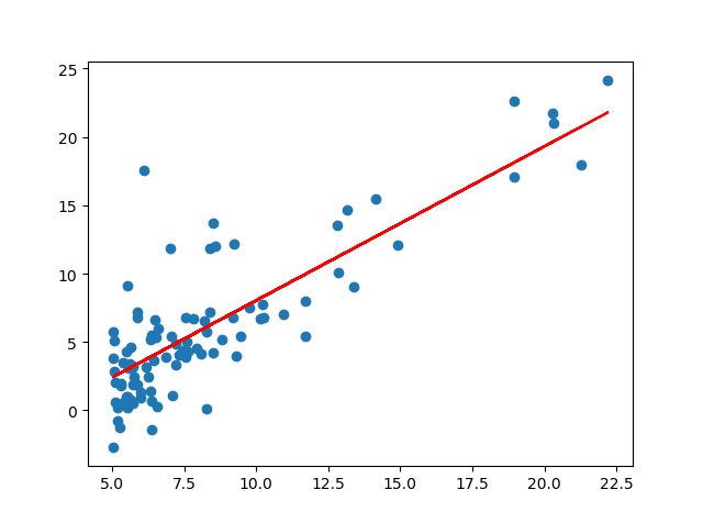
拟合的图像:
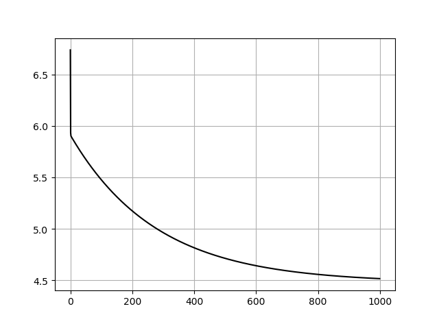
代价训练记录:
实验中遇到的问题主要是numpy模块对于矩阵和向量的操作有些生疏,其他没有什么困难的地方,也没有什么trick。第二个实验是多个变量的线性回归梯度下降,方法一样,只需要多加一个矩阵维度即可,这里不做过多介绍。
完整代码
1 | import numpy as np |